克罗内克积 🍉

数学上,克罗内克积(Kronecker product)是两个任意大小的矩阵间的运算,表示为⊗ 。克罗内克积是外积从向量到矩阵的推广,也是张量积在标准基下的矩阵表示。 本文来自维基百科(需科学上网)。
外积(英语:Outer product),在线性代数中一般指两个向量的张量积,其结果为一矩阵;与外积相对,两向量的内积结果为标量。 外积也可视作是矩阵的克罗内克积的一种特例。
在数学中,张量积,记为 ⊗ ,可以应用于不同的上下文中,如向量、矩阵、张量、向量空间、代数、拓扑向量空间和模。在各种情况下这个符号的意义是同样的:最一般的双线性运算。
尽管没有明显证据证明德国数学家利奥波德·克罗内克是第一个定义并使用这一运算的人,克罗内克积还是以其名字命名。确实,在历史上,克罗内克积曾以Johann Georg Zehfuss名字命名为Zehfuss矩阵。
定义
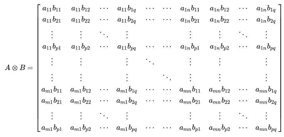
如果A是一个 m × n 的矩阵,而B是一个 p × q 的矩阵,克罗内克积$A \otimes B$ 则是一个 mp × nq 的分块矩阵
$$
A \otimes B=\left[\begin{array}{ccc}{a_{11} B} & {\cdots} & {a_{1 n} B} \ {\vdots} & {\ddots} & {\vdots} \ {a_{m 1} B} & {\cdots} & {a_{m n} B}\end{array}\right]
$$
在数学的矩阵理论中,一个分块矩阵或是分段矩阵就是将矩阵分割出较小的矩形矩阵,这些较小的矩阵就称为区块。换个方式来说,就是以较小的矩阵组合成一个矩阵。
更具体地可表示为
我们可以更紧凑地写为 
例子
$$
\left[\begin{array}{ll}{1} & {2} \ {3} & {1}\end{array}\right] \otimes\left[\begin{array}{cc}{0} & {3} \ {2} & {1}\end{array}\right]=\left[\begin{array}{llll}{1 \cdot 0} & {1 \cdot 3} & {2 \cdot 0} & {2 \cdot 3} \ {1 \cdot 2} & {1 \cdot 1} & {2 \cdot 2} & {2 \cdot 1} \ {3 \cdot 0} & {3 \cdot 3} & {1 \cdot 0} & {1 \cdot 3} \ {3 \cdot 2} & {3 \cdot 1} & {1 \cdot 2} & {1 \cdot 1}\end{array}\right]=\left[\begin{array}{llll}{0} & {3} & {0} & {6} \ {2} & {1} & {4} & {2} \ {0} & {9} & {0} & {3} \ {6} & {3} & {2} & {1}\end{array}\right]
$$
$$
\left[\begin{array}{ll}{1} & {2} \ {3} & {4}\end{array}\right] \otimes\left[\begin{array}{ll}{0} & {5} \ {6} & {7}\end{array}\right]=\left[\begin{array}{lll}{1} & {0} & {5} \ {6} & {7} & {2} \ {3} & {\left[\begin{array}{ll}{0} & {5} \ {6} & {7}\end{array}\right]} & {4\left[\begin{array}{ll}{0} & {5} \ {6} & {7}\end{array}\right]}\end{array}\right]=\left[\begin{array}{lllll}{1 \times 0} & {1 \times 5} & {2 \times 0} & {2 \times 5} \ {1 \times 6} & {1 \times 7} & {2 \times 6} & {2 \times 7} \ {3 \times 0} & {3 \times 5} & {4 \times 0} & {4 \times 5} \ {3 \times 6} & {3 \times 7} & {4 \times 6} & {4 \times 7}\end{array}\right]=\left[\begin{array}{cccc}{0} & {5} & {0} & {10} \ {6} & {7} & {12} & {14} \ {0} & {15} & {0} & {20} \ {18} & {21} & {24} & {28}\end{array}\right]
$$
特性
双线性和结合律
克罗内克积是张量积的特殊形式,因此满足双线性与结合律:
$$
\begin{array}{l}{A \otimes(B+C)=A \otimes B+A \otimes C \quad \text { (if } B \text { and } C \text { have the same size) }} \ {(A+B) \otimes C=A \otimes C+B \otimes C \quad \text { (if } A \text { and } B \text { have the same size) }} \ {(k A) \otimes B=A \otimes(k B)=k(A \otimes B)} \ {(A \otimes B) \otimes C=A \otimes(B \otimes C)}\end{array}
$$
其中,A, B 和 C 是矩阵,而 k 是常量。
克罗内克积不符合交换律:通常,$A \otimes B$ 不同于 $B \otimes A$ 。
$A \otimes B$ 和是$B \otimes A$排列等价的,也就是说,存在排列矩阵P和Q,使得
$$
A \otimes B=P(B \otimes A) Q
$$
如果A和B是方块矩阵,则$A \otimes B$ 和$B \otimes A$甚至是排列相似的,也就是说,我们可以取P = QT。
混合乘积性质
如果A、B、C和D是四个矩阵,且矩阵乘积AC和BD存在,那么:
$$
(\mathbf{A} \otimes \mathbf{B})(\mathbf{C} \otimes \mathbf{D})=\mathbf{A} \mathbf{C} \otimes \mathbf{B D}
$$
这个性质称为“混合乘积性质”,因为它混合了通常的矩阵乘积和克罗内克积。于是可以推出,$A \otimes B$ 是可逆的当且仅当A和B是可逆的,其逆矩阵为:
$$
(\mathbf{A} \otimes \mathbf{B})^{-1}=\mathbf{A}^{-1} \otimes \mathbf{B}^{-1}
$$
克罗内克和
如果A是n × n矩阵,B是m × m矩阵,$\mathbf{I}{k}$表示k × k单位矩阵,那么我们可以定义克罗内克和$\otimes $为:
$$
\mathbf{A} \oplus \mathbf{B}=\mathbf{A} \otimes \mathbf{I}{m}+\mathbf{I}_{n} \otimes \mathbf{B}
$$
谱
假设A和B分别是大小为n和q的方块矩阵。设λ1,……,λn为A的特征值,μ1,……,μq为B的特征值。那么$A \otimes B$的特征值为:
$$
\lambda_{i} \mu_{j}, \quad i=1, \ldots, n, j=1, \ldots, q
$$
于是可以推出,两个矩阵的克罗内克积的迹和行列式为:
$$
\operatorname{tr}(\mathbf{A} \otimes \mathbf{B})=\operatorname{tr} \mathbf{A} \operatorname{tr} \mathbf{B} \quad \text { and } \quad \operatorname{det}(\mathbf{A} \otimes \mathbf{B})=(\operatorname{det} \mathbf{A})^{q}(\operatorname{det} \mathbf{B})^{n}
$$
奇异值
如果A和B是长方矩阵,那么我们可以考虑它们的奇异值。假设A有rA个非零的奇异值,它们是:
$$
\sigma_{\mathbf{A}, i}, \quad i=1, \dots, r_{\mathbf{A}}
$$
类似地,设B的非零奇异值为:
$$
\sigma_{\mathbf{B}, i}, \quad i=1, \dots, r_{\mathbf{B}}
$$
那么克罗内克积$A \otimes B$有个$r_{\mathbf{A}} r_{\mathbf{B}}$非零奇异值,它们是:
$$
\sigma_{\mathbf{A}, i} \sigma_{\mathbf{B}, j}, \quad i=1, \ldots, r_{\mathbf{A}}, j=1, \ldots, r_{\mathbf{B}}
$$
由于一个矩阵的秩等于非零奇异值的数目,因此我们有:
$$
\operatorname{rank}(\mathbf{A} \otimes \mathbf{B})=\operatorname{rank} \mathbf{A} \operatorname{rank} \mathbf{B}
$$
与抽象张量积的关系
矩阵的克罗内克积对应于线性映射的抽象张量积。特别地,如果向量空间V、W、X和Y分别具有基{v1, … , vm}、 {w1, … , wn}、{x1, … , xd}和{y1, … , ye},且矩阵A和B分别在恰当的基中表示线性变换S : V → X和T : W → Y,那么矩阵A ⊗ B表示两个映射的张量积S ⊗ T : V ⊗ W → X ⊗ Y,关于V ⊗ W的基{v1 ⊗ w1, v1 ⊗ w2, … , v2 ⊗ w1, … , vm ⊗ wn}和X ⊗ Y的类似基。[1]
与图的乘积的关系
两个图的邻接矩阵的克罗内克积是它们的张量积图的邻接矩阵。两个图的邻接矩阵的克罗内克和,则是它们的笛卡儿积图的邻接矩阵。参见[2]第96个练习的答案。
转置
克罗内克积转置运算符合分配律:
$$
(A \otimes B)^{T}=A^{T} \otimes B^{T}
$$
矩阵方程
克罗内克积可以用来为一些矩阵方程得出方便的表示法。例如,考虑方程AXB = C,其中A、B和C是给定的矩阵,X是未知的矩阵。我们可以把这个方程重写为
$$
\left(B^{T} \otimes A\right) \operatorname{vec}(X)=\operatorname{vec}(A X B)=\operatorname{vec}(C)
$$
这样,从克罗内克积的性质可以推出,方程AXB = C具有唯一的解,当且仅当A和B是非奇异矩阵。(Horn & Johnson 1991,Lemma 4.3.1).
在这里,vec(X)表示矩阵X的向量化,它是把X的所有列堆起来所形成的列向量。
如果把X的行堆起来,形成列向量x,则$A X B$也可以写为$\left(A \otimes B^{T}\right) x$(Jain 1989,2.8 block Matrices and Kronecker Products)。
参考文献
- ^ Pages 401–402 of Dummit, David S.; Foote, Richard M., Abstract Algebra 2, New York: John Wiley and Sons, Inc., 1999, ISBN 0-471-36857-1
- ^ D. E. Knuth: “Pre-Fascicle 0a: Introduction to Combinatorial Algorithms”, zeroth printing (revision 2), to appear as part of D.E. Knuth: The Art of Computer Programming Vol. 4A
- Horn, Roger A.; Johnson, Charles R., Topics in Matrix Analysis, Cambridge University Press, 1991, ISBN 0-521-46713-6.
- Jain, Anil K., Fundamentals of Digital Image Processing, Prentice Hall, 1989, ISBN 0-13-336165-9.
- https://www.wikiwand.com/zh-cn/%E5%85%8B%E7%BD%97%E5%86%85%E5%85%8B%E7%A7%AF
- https://www.wikiwand.com/en/Kronecker_product
- Horn, Roger A.; Johnson, Charles R. (1991), [*Topics in Matrix Analysis*](https://books.google.com/?id=LeuNXB2bl5EC&printsec=frontcover&dq=isbn:9780521467131#v=onepage&q="Kronecker product”&f=false), Cambridge University Press, ISBN 978-0-521-46713-1.
- Jain, Anil K. (1989), Fundamentals of Digital Image Processing, Prentice Hall, ISBN 978-0-13-336165-0.
- Steeb, Willi-Hans (1997), Matrix Calculus and Kronecker Product with Applications and C++ Programs, World Scientific Publishing, ISBN 978-981-02-3241-2
- Steeb, Willi-Hans (2006), [*Problems and Solutions in Introductory and Advanced Matrix Calculus*](https://books.google.com/?id=CSDbVU1Eg3UC&printsec=frontcover&dq=isbn:9789812569165#v=onepage&q="Kronecker product”&f=false), World Scientific Publishing, ISBN 978-981-256-916-5